3D點雲的最小二乘法求解-Python實現 | LKY 只有原創內容的 Blog

仿造各種 Python 機器學習類別的風格，建立一個 class，並且實作 fit() 與 predict() 方法。

class LeastSq3D:
  def __init__(self):
      self.coeficient = None
  
  def fit(self, pts):
  
  def predict(self, pts):

pts 就是所有的三維點，pts[0] 就是第一個點，pts[0][0] 就是第一個點的 x 座標，依此類推。

fit()

就是重現上一篇文章以 Ax=b 求解的過程。

首先初始化矩陣 A

A = [
 [x^2 + xy + 1],
 [xy + y^2 + 1],
 [x + y + 1]
]

m11 = np.sum(pts[:, 0] * pts[:, 0])
m12 = np.sum(pts[:, 0] * pts[:, 1])
m13 = np.sum(pts[:, 0])
m21 = m12
m22 = np.sum(pts[:, 1] * pts[:, 1])
m23 = np.sum(pts[:, 1])
m31 = m13
m32 = m23
m33 = pts.shape[0]
A = np.array([[m11, m12, m13], [m21, m22, m23], [m31, m32, m33]])

再來初始化矩陣 b

b = [xz, yz, z]

b1 = np.sum(pts[:, 0] * pts[:, 2])
b2 = np.sum(pts[:, 1] * pts[:, 2])
b3 = np.sum(pts[:, 2])
b = np.array([b1, b2, b3])

最後求A的反矩陣，並且乘上 b，就是最後的結果，把係數 A,B,C 存在 self.coeficient 。

self.coeficient = np.dot(np.linalg.inv(A), b)

NumPy 還提供了更強的實現

self.coeficient = np.linalg.solve(A, b)

predict()

這個部分最簡單，就是把所有的點帶入方程式，得到預測的 z 座標。

就只是寫 z = Ax + By + C。

不過要注意的是，最好用向量化寫法，不要用迴圈，這樣會比較快。

def predict(self, pts):
    if self.coeficient is None:
        raise Exception('You need to fit the model first.')
    pts = np.array(pts)
    return np.dot(pts, self.coeficient)

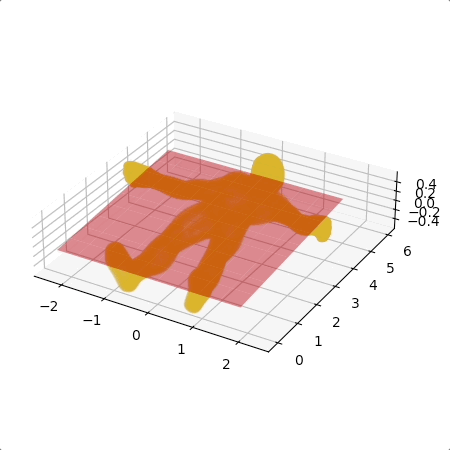
範例

我用 Free3D 的一個人體模型來做範例。

if __name__ == '__main__':
    # 載入已經讀好的點雲
    pts = np.load(r'human_body_vertices.npy')
    
    # 畫出半透明的原始點雲
    fig = plt.figure()
    ax = fig.add_subplot(111, projection='3d')
    ax.set_box_aspect(aspect = (1, 1, 0.25))
    ax.scatter(pts[:, 0], pts[:, 1], pts[:, 2], alpha=0.1, c='goldenrod')

    # 用最小二乘法求解
    l3d = LeastSq3D()
    l3d.fit(pts)

    # 對平面點雲取樣，並畫出
    x_range = np.arange(pts[:, 0].min(), pts[:, 0].max(), pts[:, 0].ptp()/10)
    y_range = np.arange(pts[:, 1].min(), pts[:, 1].max(), pts[:, 1].ptp()/10)
    xx, yy = np.meshgrid(x_range, y_range)
    zz = l3d.predict(np.array([xx.flatten(), yy.flatten(), np.ones(shape=len(xx.flatten()))]).T).reshape(xx.shape)
    ax.plot_surface(xx, yy, zz, alpha=0.5, color='r')
    plt.show()